210805_1(머신러닝)

준비물

 

 

1. 아나콘다 설치

2. 아나콘다 명령창을 이용해서 가상공간 생성

>conda create -n tensorflow python=3.6 (tensorflow라는 이름으로 파이선 3.6에 맞춰생성)

  --참고 가상공간제거 : conda remove --name tensorflow --all

오류시 해결법 : 경로를 못찾는 404 에러가뜨면

anaconda navigator에서 environments - channels - defaults 만 남기고 나머지는 삭제  

3. 가상공간 활성화

>activate tensorflow // 활성화

  -- 참고 비활성화 명령어 : deactivate

4. 파이썬 설치 관리자 업데이트

>pip install --ignore-installed --upgrade (안됨왜)

>pip install tensorflow==1.6

5. 작동확인

>python

>import tensorflow as tf

 hello = tf.constant('hello tensorflow !!!!')

sess = tf.Session()

>>> sess = tf.Session()
2021-08-05 11:26:58.535134: I C:\tf_jenkins\workspace\rel-win\M\windows\PY\36\tensorflow\core\platform\cpu_feature_guard.cc:140] Your CPU supports instructions that this TensorFlow binary was not compiled to use: AVX2

--해결법

>>> import os
>>> os.environ['TF_CPP_MIN_LOG_LEVEL'] = '2'

>>> print(sess.run(hello))
b'hello tensorflow !!!!' ---> 출력되면 성공

 

 

---

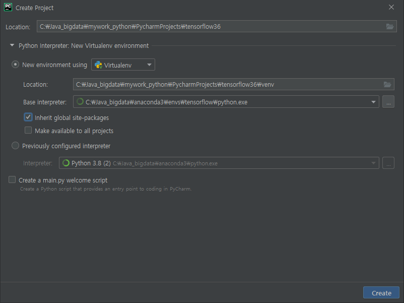
파이참에서 프로젝트생성시 위에 만든 가상공간으로 설정

 

import os
os.environ['TF_CPP_MIN_LOG_LEVEL'] = '2'

import tensorflow as tf
hello = tf.constant('hello tensorflow !!!')
sess = tf.Session()
print(sess.run(hello))
'''
b'hello tensorflow !!!'
'''

머신러닝이란?

기계 학습 또는 머닝 서닝(machine learning)은 인공지능의 한 분야로, 컴퓨터가 학습할 수 있도록 하는 알고리즘과 기술을 개발하는 분야를 말한다. 가령, 기계 학습을 통해서 수신한 이메일이 스팸인지 아닌지를 구분할 수 있도록 훈련할 수 있다.

 

기계 학습의 핵심은 표현(representation)과 일반화(generalization)에 있다

 

 

matplotlib 설치

#
import os
os.environ['TF_CPP_MIN_LOG_LEVEL']='3'

import tensorflow as tf
from tensorflow.examples.tutorials.mnist import input_data

#Data set loading
mnist = input_data.read_data_sets("./sample/MNIST/", one_hot=True)
### 학습할 손글씨 이미지 다운로드하여 저장
################### 위에 실행하고 아래진행
import tensorflow as tf
from tensorflow.examples.tutorials.mnist import input_data

mnist = input_data.read_data_sets("./sample/MNIST/", one_hot=True)
# y=wx+b
# 결과y = 가중치W * 입력값x + 절편b
# 즉, w의 값에 따라서 선형그래프의 오차값이 작은 것을 찾아 가는 것
# =선형회구

#Set up model
#x는 학습할 데이터 placeholder 미리 변수를 잡는다.float 4바이트짜리실수.
# 28*28 를 한줄로 => 784열 : 이미지 사이즈
x = tf.placeholder(tf.float32,[None, 784])
# 가중치 입력값이 784이면 , 출력은 10개(0~9사이의값)다.
W = tf.Variable(tf.zeros([784,10]))
# 절편값 : 가중치의 출력 갯수와 같다
b = tf.Variable(tf.zeros([10]))

# 공식 --- 결과y = 가중치W * 입력값x + 절편b
# 더욱 정확한 결과를 도출하기 위한 함수 softmax(), matmul(x,W) 행렬곱
# y는 내가 구한결과
y = tf.nn.softmax(tf.matmul(x, W)+b)
# y_ 라벨 : 정답..? 10개(0~9사이의값)
y_ = tf.placeholder(tf.float32,[None, 10])
# 오타들의 합이 가장 작아지도록 찾는것 비용곡선(log(y))
cross_entropy = -tf.reduce_sum(y_*tf.log(y))
# 학습 노드 비용의 합계가 가장 작은 지점을 찾는것 학습
train_step = tf.train.GradientDescentOptimizer(0.01).minimize(cross_entropy)

# 학습실행
#Session
# 전역변수 준비 및 초기화
init = tf.global_variables_initializer()
# 모든 실제 실행은 세션에서 일어난다
sess = tf.Session()
sess.run(init) # 초기화

#Learning
for i in range(1000): # 0~999
    batch_xs, batch_ys = mnist.train.next_batch(100)
    sess.run(train_step, feed_dict={x:batch_xs, y_:batch_ys})

#Validation 예측하기   tf.equal(결과치, 라벨값)
correct_prediction = tf.equal(tf.argmax(y,1), tf.argmax(y_,1))
accuracy = tf.reduce_mean(tf.cast(correct_prediction, tf.float32))

# Result should be approximately 91%. 결과 출력하기
print(sess.run(accuracy, feed_dict={x:mnist.test.images, y_:mnist.test.labels}))

#0.9178

############################# 선형회귀
## linear_regression

# set_random_seed()
# 모든 연산에 의해 생성된 난수 시퀀드를이 세션간
# 반복이 가능하게 하기위해서, 그래프 수준의 시드를 설정합니다.
# 세션이 달라도 동일한 패턴이 반복된다

# random_normal() : 임의의 값을 부여하는데 표준분포 곡선을 따른다

#Lab 2 Linear Regression

import tensorflow as tf
tf.set_random_seed(777) # for reproiducibility

# X and Y data 학습할 데이타의 부여
x_train = [1,2,3]
y_train = [1,2,3]

#try ro find values for W and b to compute y_data * W + b
# We know that W should be 1 and b should be 0
# But let Tensorflow figure it out
# Variable 텐서 플로우가 자체적으로 사용하는 변수 / 이름 = weight. 값은 1차원 배열
W= tf.Variable(tf.random_normal([1]), name='weight')
b = tf.Variable(tf.random_normal([1]),name='bias')

#Our hypothesis XW+b 가성 공식 = 입력 * 가중치 + 초기값
hypothesis = x_train * W + b

#cost/loss function 비용구함 = 평균(제곱(기대갑-입력값))
cost = tf.reduce_mean(tf.square(hypothesis - y_train))

#  Minimize GradientDecsentOptimizer을 사용해서 비용을 최소화 시킨다.
optimizer = tf.train.GradientDescentOptimizer(learning_rate=0.01)

# 시작 노드의 이름을 train
train = optimizer.minimize(cost)

# Launch the graph in a session 실행하기위한 세션을 생성
sess= tf.Session()
#Initializes global variables in the graph : 전역변수 초기화를 시켜 실행
sess.run(tf.global_variables_initializer())

# Fit the line 학습횟수 2000회
for step in range(2001):
    sess.run(train)
    if step % 20 == 0: #20번째 마다 단계, 비용 cost, 가중치 weight, 초기값 bias를 출력해봄
        print(step,sess.run(cost),sess.run(W),sess.run(b))

# y_data = x_data * W + b
#      1 =      1 * W + b 이공식을 성립시킬수 있는 W와 b는 얼마일까?
# 비용이 점점 작아지고 / 가중치는 1에 수렴하며, 초기값은 0 에 가까워짐을 알 수 있다.

# Learns best fit W:[1.], b:[0.]
'''
0 2.823292 [2.1286771] [-0.8523567]
20 0.19035067 [1.533928] [-1.0505961]
40 0.15135698 [1.4572546] [-1.0239124]
60 0.1372696 [1.4308538] [-0.9779527]
'''
'''
1940 1.6119748e-05 [1.0046631] [-0.01060018]
1960 1.4639714e-05 [1.004444] [-0.01010205]
1980 1.3296165e-05 [1.0042351] [-0.00962736]
2000 1.20760815e-05 [1.0040361] [-0.00917497]
'''

 

# Lab2 linear_regression
import  tensorflow as tf
tf.set_random_seed(777) # for reproducibility

# Try to find values for W and b to compute y_data = W * x_data + b
# We know that W should be 1 and b should be 0
# But let's use TensorFlow to figure it out
W= tf.Variable(tf.random_normal([1]),name='weight')
b = tf.Variable(tf.random_normal([1]),name='bias')

#Now we can use X and Y in place of x_data and y_data
# # placeholders for a tensor that will be always fed using feed_dict
# shape=[None]은 차후 입력되는 인자의 갯수가 상관없음을 나타낸다
#값을 미리 주지 않고 placeholder를 통해서 설정하고 나중에 실제 값을 부여할 수 있도록함
X = tf.placeholder(tf.float32, shape=[None])
Y = tf.placeholder(tf.float32, shape=[None])

#Out hypothesis CW +b
hypothesis = X * W + b

#cost/loss function
cost = tf.reduce_mean(tf.square(hypothesis - Y))

# Minimize 기울기가 하방으로 내려가는 최적화
optimizer = tf.train.GradientDescentOptimizer(learning_rate=0.01)
train = optimizer.minimize(cost)

#Launch the graph in a session.
sess = tf.Session()
# initializes global variables in the graph.
sess.run(tf.global_variables_initializer())

# Fit the line 위에서 placeholder 를 통한값을 feed_dict 으로 실제 부여함
for step in range(2001):
    cost_val, W_val, b_val,_=\
    sess.run([cost,W,b,train], feed_dict={X:[1,2,3],Y:[1,2,3]})
    if step % 20 == 0:
        print(step, cost_val, W_val, b_val)
# # Learns best fit W:[1], b:[0]
'''
1960 1.4711059e-05 [1.004444] [-0.01010205]
1980 1.3360998e-05 [1.0042351] [-0.00962736]
2000 1.21343355e-05 [1.0040361] [-0.00917497]
'''

# # Testring out model
print(sess.run(hypothesis, feed_dict={X:[5]}))
print(sess.run(hypothesis, feed_dict={X:[2.5]}))
print(sess.run(hypothesis, feed_dict={X:[1.5,3.5]}))
'''
[5.0110054]
[2.500915]
[1.4968792 3.5049512]
'''

#Fit the line with new training data
# 입력 -X:[1,2,3,4,5] 라벨 -Y:[2.1,3.1,4.1,5.1,6.1] 처럼 되도록 학습시킨다
for step in range(2001):
    cost_val,W_val,b_val,_ = \
        sess.run([cost,W,b,train],feed_dict={X:[1,2,3,4,5],Y:[2.1,3.1,4.1,5.1,6.1]})
    if step % 20 == 0:
        print(step,cost_val,W_val,b_val)
'''
1960 1.3700877e-06 [1.0007573] [1.0972656]
1980 1.1968872e-06 [1.0007079] [1.0974445]
2000 1.0450387e-06 [1.0006615] [1.0976118]
'''
#Testing our model
# 학습된 결과에 의거하여 X값을 입력하면 결과 Y는 얼마라고 예측하는가?
print(sess.run(hypothesis, feed_dict={X:[5]}))
print(sess.run(hypothesis, feed_dict={X:[2.5]}))
print(sess.run(hypothesis, feed_dict={X:[1.5,3.5]}))
'''
[6.1009192]
[3.5992656]
[2.5986042 4.599927 ]
'''