20812_01(머신러닝)
# xor 문제와 퍼셉트론
# (퍼셉트론+퍼셉트론+퍼셉트론) 딥러닝의 대두

#Lab 9 XOR AND OR
# XOR를 logistic regression으로 해결이 될까? 결과를 살펴보자
import tensorflow as tf
import numpy as np

tf.set_random_seed(777) # for reproducibility
learning_rate = 0.1
# 0 0 --> 0, 01 --> 1, 1 0 --> 1, 1 1 --> 0
x_data = [[0,0],[0,1],[1,0],[1,1]]
y_data = [[0],[1],[1],[0]]

x_data = np.array(x_data, dtype=np.float32)
y_data = np.array(y_data, dtype=np.float32)

X = tf.placeholder(tf.float32,[None,2])
Y = tf.placeholder(tf.float32,[None,1])

W = tf.Variable(tf.random_normal([2,1]),name='weight')
b = tf.Variable(tf.random_normal([1]),name='bias')

# Hypothesis using sigmoid : tf.div(1., 1. + tf.exp(tf.matmul(X,W))
hypo = tf.sigmoid(tf.matmul(X,W)+b)

# cost/loss function
cost = -tf.reduce_mean(Y*tf.log(hypo)+(1-Y) * tf.log(1-hypo))

train = tf.train.GradientDescentOptimizer(learning_rate=learning_rate).minimize(cost)

# Accuracy computation
# True if hypothesis > 0.5 else False
predicted = tf.cast(hypo > 0.5, dtype=tf.float32)
accuracy = tf.reduce_mean(tf.cast(tf.equal(predicted,Y), dtype=tf.float32))

# Launch graph
with tf.Session() as sess:
    sess.run(tf.global_variables_initializer())

    for step in range(10001):
        sess.run(train, feed_dict={X:x_data,Y:y_data})
        if step % 100 == 0:
            print(step,sess.run(cost,feed_dict={X:x_data,Y:y_data}), sess.run(W))
    # Accuracy report
    h,c,a = sess.run([hypo, predicted, accuracy], feed_dict={X:x_data,Y:y_data})
    print("\nHyphthesis:",h,"\nCorrect:",c,"\nAccuracy:",a)

    '''
    Hyphthesis: [[0.5]
                 [0.5]
                 [0.5]
                 [0.5]]
    Correct: [[0.]
              [0.]
              [0.]
              [0.]]
    Accuracy: 0.5 <-- 정확도가 낟음
    '''
hypo = tf.sigmoid(tf.matmul(X,W)+b)
XOR
입력값 결과(라벨) A B C
----------------------------------------------------------------------------
[0,0] 0 0 1 0
[0,1] 1 0 0 1
[1,0] 1 0 0 1
[1,1] 0 1 0 0
----------------------------------------------- 여러개의 퍼셉트론이 있는 경우
가중치(W)와 절편(b)은 임의의 값으로 지정하여 계산해 보자
(수없이 많은 반복학습을 통하여 최정의 가중치W와 절편b를 구하게 될것이다)
A: 입력 * 가중치 + bias
[0,0] * [5
5] + (-8) ==> -8 sigmoid=> 0
B : 입력 * 가중치 + bias
[0,0] * [-7
-7] + (3) ==> 3 sigmoid=> 1
--------------------------------------------- 다음단계 - 이전단계의 출력을 다음단계 입력으로
C : 입력 * 가중치 + bias
출력을
입력으로
[0,1] * [-11
-11] + (6) ==> -5 sigmoid=> 0 ===> C의 최종 출력값은 XOR의 결과와 동일하다
============================ [0,0] 만 입력해본 결과
나머지 [0,1], [1,0], [1,1] 은 계산결과가 C가 XOR와 결과 동일해지는지 확인해보자
다층퍼셉트론 ===> 뉴럴 네트워크(neural network) ===> 신경망회로 ===> 은닉층이 많아지면 딥러닝
# xor 문제와 멀티 퍼셉트론을 이용한 해결
# (퍼셉트론+퍼셉트론+퍼셉트론) 딥러닝의 대두

#Lab 9 XOR AND OR
# XOR를 logistic regression으로 해결이 될까? 결과를 살펴보자
import tensorflow as tf
import numpy as np

tf.set_random_seed(777) # for reproducibility
learning_rate = 0.1
# 0 0 --> 0, 01 --> 1, 1 0 --> 1, 1 1 --> 0
x_data = [[0,0],[0,1],[1,0],[1,1]]
y_data = [[0],[1],[1],[0]]

x_data = np.array(x_data, dtype=np.float32)
y_data = np.array(y_data, dtype=np.float32)

X = tf.placeholder(tf.float32,[None,2])
Y = tf.placeholder(tf.float32,[None,1])

# 1단계 뉴럴네트워크 neural network
W1 = tf.Variable(tf.random_normal([2,2]),name='weight1')
b1 = tf.Variable(tf.random_normal([2]),name='bias1')
layer1 = tf.sigmoid(tf.matmul(X,W1)+b1)

# 2단계 뉴럴 네트워크 neural network 1단계 층을 추가하고 확인해보자 XOR는 해결이 가능한가
W2 = tf.Variable(tf.random_normal([2,1]),name='weight2')
b2 = tf.Variable(tf.random_normal([1]),name='bias2')
hypo = tf.sigmoid(tf.matmul(layer1,W2)+b2)

# cost/loss function
cost = -tf.reduce_mean(Y*tf.log(hypo)+(1-Y) * tf.log(1-hypo))

train = tf.train.GradientDescentOptimizer(learning_rate=learning_rate).minimize(cost)

# Accuracy computation
# True if hypothesis > 0.5 else False
predicted = tf.cast(hypo > 0.5, dtype=tf.float32)
accuracy = tf.reduce_mean(tf.cast(tf.equal(predicted,Y), dtype=tf.float32))

# Launch graph
with tf.Session() as sess:
    sess.run(tf.global_variables_initializer())

    for step in range(10001):
        sess.run(train, feed_dict={X:x_data,Y:y_data})
        if step % 100 == 0:
            print(step,sess.run(cost,feed_dict={X:x_data,Y:y_data}), sess.run([W1,W2]))
    # Accuracy report
    h,c,a = sess.run([hypo, predicted, accuracy], feed_dict={X:x_data,Y:y_data})
    print("\nHyphthesis:",h,"\nCorrect:",c,"\nAccuracy:",a)

'''
Hyphthesis: [[0.01338218]
 [0.98166394]
 [0.98809403]
 [0.01135799]]
Correct: [[0.]
 [1.]
 [1.]
 [0.]]
Accuracy: 1.0 <- 정확도가 올라갔다.
'''
# xor 문제와 멀티 퍼셉트론을 이용한 해결
# (퍼셉트론+퍼셉트론+퍼셉트론) 딥러닝의 대두

#Lab 9 XOR
# XOR를 logistic regression으로 해결이 될까? 결과를 살펴보자
import tensorflow as tf
import numpy as np

tf.set_random_seed(777) # for reproducibility
learning_rate = 0.1
# 0 0 --> 0, 01 --> 1, 1 0 --> 1, 1 1 --> 0
x_data = [[0,0],[0,1],[1,0],[1,1]]
y_data = [[0],[1],[1],[0]]

x_data = np.array(x_data, dtype=np.float32)
y_data = np.array(y_data, dtype=np.float32)

X = tf.placeholder(tf.float32,[None,2])
Y = tf.placeholder(tf.float32,[None,1])

# laer를 여러층을 두어 깊게 만들고, 출력을 여러개(아래는10)로 하여 넓게 만들어서 XOR 해결해보자
# XOR를 더 잘 해결한다
# 1단계 - 2 입력 10 출력
W1 = tf.Variable(tf.random_normal([2,10]),name='weight1')
b1 = tf.Variable(tf.random_normal([10]),name='bias1')
layer1 = tf.sigmoid(tf.matmul(X,W1)+b1)
# 2단계 - 10 입력 10 출력
W2 = tf.Variable(tf.random_normal([10,10]),name='weight2')
b2 = tf.Variable(tf.random_normal([10]),name='bias2')
layer2 = tf.sigmoid(tf.matmul(layer1,W2)+b2)
# 3단계 - 10 입력 1 0출력
W3 = tf.Variable(tf.random_normal([10,10]),name='weight3')
b3 = tf.Variable(tf.random_normal([10]),name='bias3')
layer3 = tf.sigmoid(tf.matmul(layer2,W3)+b3)
# 4단계 - 10 입력 1 출력
W4 = tf.Variable(tf.random_normal([10,1]),name='weight4')
b4 = tf.Variable(tf.random_normal([1]),name='bias4')
hypo = tf.sigmoid(tf.matmul(layer3,W4)+b4)

# cost/loss function
cost = -tf.reduce_mean(Y*tf.log(hypo)+(1-Y) * tf.log(1-hypo))

train = tf.train.GradientDescentOptimizer(learning_rate=learning_rate).minimize(cost)

# Accuracy computation
# True if hypothesis > 0.5 else False
predicted = tf.cast(hypo > 0.5, dtype=tf.float32)
accuracy = tf.reduce_mean(tf.cast(tf.equal(predicted,Y), dtype=tf.float32))

# Launch graph
with tf.Session() as sess:
    sess.run(tf.global_variables_initializer())

    for step in range(10001):
        sess.run(train, feed_dict={X:x_data,Y:y_data})
        if step % 100 == 0:
            print(step,sess.run(cost,feed_dict={X:x_data,Y:y_data}), sess.run([W1,W2]))
    # Accuracy report
    h,c,a = sess.run([hypo, predicted, accuracy], feed_dict={X:x_data,Y:y_data})
    print("\nHyphthesis:",h,"\nCorrect:",c,"\nAccuracy:",a)
'''
Hyphthesis: [[0.5]
             [0.5]
             [0.5]
             [0.5]]
Correct: [[0.]
          [0.]
          [0.]
          [0.]]
Accuracy: 0.5 <-- 정확도가 낟음
'''
'''
Hyphthesis: [[0.01338218]
 [0.98166394]
 [0.98809403]
 [0.01135799]]
Correct: [[0.]
 [1.]
 [1.]
 [0.]]
Accuracy: 1.0 <- 정확도가 올라갔다.
'''
'''
Hyphthesis: [[7.8051287e-04]
 [9.9923813e-01]
 [9.9837923e-01]
 [1.5565894e-03]]
Correct: [[0.]
 [1.]
 [1.]
 [0.]]
Accuracy: 1.0 <- 역시 정확도가 높다
출력은 안했지만 비용또한 2층구조에 비해 많이 낮아졌다
'''
import tensorflow as tf
import numpy as np

tf.set_random_seed(777) # for reproducibility
learning_rate = 0.1
# 0 0 --> 0, 01 --> 1, 1 0 --> 1, 1 1 --> 0
x_data = [[0,0],[0,1],[1,0],[1,1]]
y_data = [[0],[1],[1],[0]]

x_data = np.array(x_data, dtype=np.float32)
y_data = np.array(y_data, dtype=np.float32)

X = tf.placeholder(tf.float32,[None,2],name='x-input')
Y = tf.placeholder(tf.float32,[None,1],name='y-input')

with tf.name_scope("layer1") as scope:
    W1 = tf.Variable(tf.random_normal([2,2]),name='weight1')
    b1 = tf.Variable(tf.random_normal([2]),name='bias1')
    layer1 = tf.sigmoid(tf.matmul(X,W1)+b1)

    w1_hist = tf.summary.histogram("weight1",W1)
    b1_hist = tf.summary.histogram("biases1",b1)
    layer1_hist = tf.summary.histogram("layer1",layer1)

with tf.name_scope("layer2") as scope:
    W2 = tf.Variable(tf.random_normal([2, 1]), name='weight2')
    b2 = tf.Variable(tf.random_normal([1]), name='bias2')
    hypothesis = tf.sigmoid(tf.matmul(layer1, W2) + b2)

    w2_hist = tf.summary.histogram("weight2", W2)
    b2_hist = tf.summary.histogram("biases2", b2)
    hypothesis_hist = tf.summary.histogram("hypothesis", hypothesis)

# cost/loss function
with tf.name_scope("cost") as scope:
    cost = -tf.reduce_mean(Y*tf.log(hypothesis)+(1-Y)*tf.log(1-hypothesis))
    cost_summ = tf.summary.scalar("cost",cost)

with tf.name_scope("train") as scope:
    train = tf.train.AdamOptimizer(learning_rate=learning_rate).minimize(cost)

# Accuracy compulation
# True if hypothesis >  0.5 else False
predicted = tf.cast(hypothesis> 0.5, dtype=tf.float32)
accuracy = tf.reduce_mean(tf.cast(tf.equal(predicted,Y), dtype=tf.float32))
accuracy_summ = tf.summary.scalar("accuracy",accuracy)

#Launch graph
with tf.Session() as sess:
     # tensorboard -- logdir = ./logs/xor_logs
    merged_summary = tf.summary.merge_all()
    writer = tf.summary.FileWriter("./logs/xor_logs_r1_01")
    writer.add_graph(sess.graph) # show the graph

    '''
    tensorboard 실행시키기
    (tensorflow) C:Users\myhome>tensorboard -- logdir = C:\ProgramData\Anaconda3\envs\
    tensorflow\본인작업경로\logs
    Starting TensorBoard b'47' at http://0.0.0.0:6006
    (Press CTRL+C to quit)
    마지막 웹브라우저를 열고 http://localhost:6006/ 접근해보자

    안될때
    1. anaconda 명령창을 열고 tensorflow 가상공간 활설화
    >activate tensorflow
    2.(tensorflow) C:Users\myhome>tensorboard -- logdir = C:\ProgramData\Anaconda3\envs\
    tensorflow\본인작업경로\logs
    3. 명령창에서 보여주는 웹주소 경로를 복사하여 브라우저에서 접속한다
    '''

    #Initialize TensorFlow variables
    sess.run(tf.global_variables_initializer())

    for step in range(10001):
        summary,_ = sess.run([merged_summary,train], feed_dict={X:x_data,Y:y_data})
        writer.add_summary(summary, global_step=step)

        if step % 100 == 0:
            print(step,sess.run(cost,feed_dict={X:x_data,Y:y_data}),sess.run([W1,W2]))

    #Accuracy report
    h, c, a = sess.run([hypothesis,predicted,accuracy], feed_dict={X:x_data,Y:y_data})
    print("\nHypothesis:",h,"\nCorrect:",c,"\nAccuracy:",a)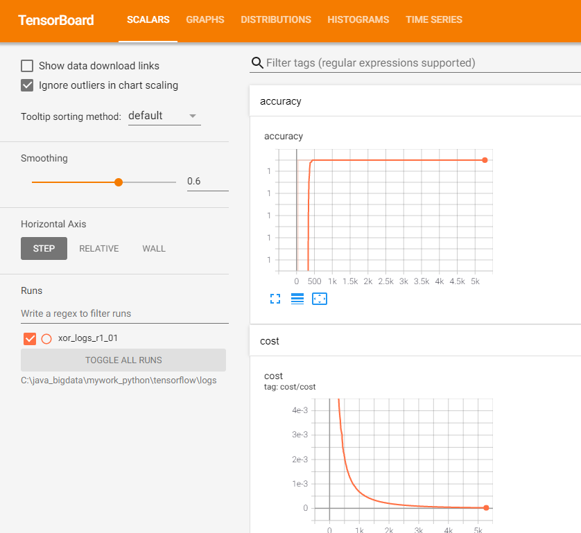
# 오차를 감소 시키지 위한 방안
# 오차의 역전파 -- 오차를 역으로 전파한다. back propagation
# 원리만 이해해보자

'''
1단계
    hypo = X * W + b : X * W + b ===> hypo
        오차 : 라벨 - 예측값 : Y - hypo == Error 의 크기
         최종오차는 = 가중치 오차 + 절편 오차 + 입력값오차 <===
         전체 오차 = 각각의 오차의 합계와 같다 ===> 편미분이 적용된다다
        Error를 뒤로 보내서 W에서 발생하는 오차를 새로 구하여 할당도
        b에서 발생하는 오차를 수정하여 새로운 b 구하여 할당

    그리고 다시 최종 오차를 구하기 그오차가 0이 될때까지 계속 이전의 발생요소의
     오차가 0이 될때까지 반복하는 것

    순서로 설명 - 1. 임의의 초기 가중치를 준 뒤 결과를 계산한다.
                2. 계산결과와 우리가 원하는 값 사이의 오차를 구한다
                3. 경사하강법을 이용하여 바로 앞 가중치를 오차가 작아지는 방향으로
                    업데이트 한다
                4. 1~3과정을 반복한다. 오차 더이상 줄어들지 않을때까지
                오차변화 / 가중치 변화 <=== 가중치 기울기
        공식 : 새가중치 = 현가중치 - (오차변화 / 가중치변화)
                W(t+1) = W(t) - (dE / dW)
'''
# WIP
import  tensorflow as tf

tf.set_random_seed(777)

# tf Graph Input
x_data = [[1.],[2.],[3.]]
y_data =[[1.],[2.],[3.]]

#placeholders for a tensor that will be always fed.
X = tf.placeholder(tf.float32,shape=[None,1])
Y = tf.placeholder(tf.float32,shape=[None,1])
# Set wrong model weihts
W = tf.Variable(tf.truncated_normal([1,1]))
b = tf.Variable(5.)

# Forwards prop
hypothesis = tf.matmul(X,W)+b

# diff
assert hypothesis.shape.as_list() == Y.shape.as_list()
diff = (hypothesis - Y)

# Back prop(chain rule) 결과와 라벨의 차이를
d_l1 = diff
d_b = d_l1
# transpose : 축을 서로 바꾼다
# 변호가 된다. 아래의 예는 2번 축과 3번 축을 서로 바꾸겠다라는 의미가 된다
# 활용 tf.transpose(x, perm=[0,2,1])
d_w = tf.matmul(tf.transpose(X),d_l1)

print(X,W,d_l1,d_w)
# Updating network using gradients 조절된 가중치 조절된 바이어스 값을 할당
# W = W -learning_rate * d_w 를 새로 할당 / b = b - learning_rate * tf.reduce_mean(d_b)할당
learning_rate=0.1
step = [
    tf.assign(W,W - learning_rate * d_w),
    tf.assign(b, b - learning_rate * tf.reduce_mean(d_b)),
]

# 7. Running and testing the trainging process : tf.square 제곱
RMSE = tf.reduce_mean(tf.square(Y-hypothesis))

sess = tf.InteractiveSession()
init = tf.global_variables_initializer()
sess.run(init)

for i in range(1000):
    print(i,sess.run([step,RMSE],feed_dict={X:x_data,Y:y_data}))

print(sess.run(hypothesis, feed_dict={X:x_data}))
'''
995 [[array([[0.99999714]], dtype=float32), 6.532301e-06], 6.366463e-12]
996 [[array([[0.99999726]], dtype=float32), 6.4568017e-06], 6.257513e-12]
997 [[array([[0.9999972]], dtype=float32), 6.3574607e-06], 5.783818e-12]
998 [[array([[0.99999726]], dtype=float32), 6.2779877e-06], 5.6464464e-12]
999 [[array([[0.9999973]], dtype=float32), 6.1985147e-06], 5.6464464e-12]
[[1.0000035]
 [2.0000007]
 [2.999998 ]]
'''